Next: Gravity Modeling and Inversion Up: Optimization of Non-Linear Gravity Previous: Introduction
![]()
![]()
![]()
Next: Gravity
Modeling and Inversion Up: Optimization
of Non-Linear Gravity Previous: Introduction
The application of an iterative improvement algorithm presupposes the definition of configurations, a cost function and a generation mechanism, i.e. a simple prescription to generate a transition from a configuration to another one.
The GSA method leads to the minimization of a cost function ![]() through a stochastic cooling. The procedure consists in comparing the cost
function for two random vectors
through a stochastic cooling. The procedure consists in comparing the cost
function for two random vectors ![]() (or configuration) obtained using the generalized visiting distribution.
In this sense, the hypersurface defined by
(or configuration) obtained using the generalized visiting distribution.
In this sense, the hypersurface defined by ![]() is randomly visited and the algorithm terminates when a configuration is
obtained whose cost is no worse than any of its neighbors.
is randomly visited and the algorithm terminates when a configuration is
obtained whose cost is no worse than any of its neighbors.
Differently of the gradient methods, solutions obtained by the SA, do not depend on the initial configuration and have a cost usually close to the minimum one. The simulated annealing is a technique that has attracted significant attention in a diversity of problems, especially those where a desired global extremum is hidden among many local extrema. The GSA algorithm can now be viewed as a sequence of generalized Metropolis algorithms evaluated at a sequence of decreasing values of the control parameter.
In summary, we describe the principal steps to built the numerical procedure
[5, 8]
in order to map the global minima of a function ![]() depend on of a multidimensional continuous parameter
depend on of a multidimensional continuous parameter ![]()
(i) Fix the acceptance and visiting indexes ![]() and
and ![]() (we recall that
(we recall that ![]() and (1,2) respectively correspond to the Boltzmann and Cauchy machines).
Start, at t=1, with an arbitrary value
and (1,2) respectively correspond to the Boltzmann and Cauchy machines).
Start, at t=1, with an arbitrary value ![]() and a high enough value
and a high enough value ![]() (visiting temperature) and cool as follows:
(visiting temperature) and cool as follows:
where t is the discrete time corresponding to the computer iteration.
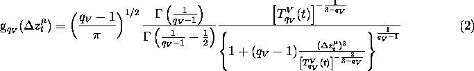
(ii) Then randomly generate each component ![]() (
( ![]() ) of
) of ![]() using the visiting distribution probability
using the visiting distribution probability ![]() given by
given by
where ![]() is the gamma function; D is the number of components of
is the gamma function; D is the number of components of ![]() . This procedure assures that the system can both escape from any local
minimum and explore the entire cost function.
. This procedure assures that the system can both escape from any local
minimum and explore the entire cost function.
(iii) Then calculate the cost function ![]() with the following conditions:
with the following conditions:
If ![]()
![]() , replace
, replace ![]() by
by ![]()
If ![]() , accept
, accept ![]() with the acceptance probability
with the acceptance probability ![]() defined by
defined by
with ![]() [5].
[5].
(iv) Calculate the new temperature ![]() using Eq.(1) and go back to (ii) until the minimum of
using Eq.(1) and go back to (ii) until the minimum of ![]() is reached within the desired precision.
is reached within the desired precision.